
From 1 to 2: Scaling Up the Qubits
Concepts #2: Multiple Qubits, Entanglement, and Live Entanglement Applications


Welcome to the second installment of Quantum Disentangled, a monthly newsletter that breaks down quantum-related concepts, analyzes cutting-edge papers, and provides research on quantum computing companies. Our goal is to publicize our macro-level quantum theses as well as to bridge the knowledge gap and become the most accessible source of quantum-related information for students, researchers, investors, and the general public. Learn about us and our backgrounds here.
Join us by subscribing here for free and have future posts delivered straight to your inbox:
If you learn something enjoy our work and want to support us, we’d appreciate you telling your friends. It helps a ton. 🫡
Key Takeaways
Physicists define a state space known as Hilbert space to understand quantum systems. The Bloch sphere described in post 1 can only represent 1 qubit.
Entanglement is another key quantum concept that can occur between multiple qubits. We can use simple algebra to demonstrate the difference between unentangled and entangled states for 2 qubits.
There are live, working experiments today that have demonstrated maximally entangled two-qubit states separated by macroscopic distances — one between space and China and the other at the University of Innsbruck in Austria.
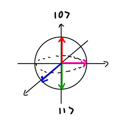
In our first post, we went over the basic building block: the qubit. We introduced the Bloch sphere, a way of visualizing the full range of possibilities of the 2-dimensional vector space for a single qubit.
However, the Bloch sphere can only be utilized for a single qubit, which isn’t all that interesting by itself. When there are multiple qubits, we can start to think about another key, nonclassical quantum property called entanglement. Let’s dive into how we can start thinking about more than 1 qubit.
Multiple Qubits
When there are multiple qubits, we cannot use the Bloch sphere because additional qubits increase the dimensionality of the state space.
For 1 qubit, the range of possibilities lies on the 2-dimensional surface of a 3-dimensional sphere. The state space has a dimensionality of 2.
For 2 qubits, the range of possibilities lies on the 4-dimensional surface of a 5-dimensional sphere. The state space has a dimensionality of 4.
For 3 qubits, the range of possibilities lies on the 8-dimensional surface of a 9-dimensional sphere. The state space has a dimensionality of 8.
And so on.
As you can start to notice, the number of computational basis states scales exponentially as 2n, where n is the number of qubits. This is also true in classical computing, but the superposition of those basis states increases the dimension of the state space that physicists call Hilbert space (for future reference — “Hilbert space” and “state space” can be used interchangeably and mean the same thing).
Since visualizing the above 3-dimensional space is hard, we can represent this space as existing inside an arbitrary polygon.
For the single qubit example, this is what the Hilbert space looks like:
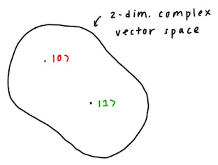
The two points |0⟩ and |1⟩ represent the two poles of the original Bloch sphere, which correspond to the classical states (0 and 1). Each other possible point within the Hilbert space (circular blob) simply represents another point along the sphere.
In turn, we can use this same Hilbert space representation to visualize a 2-qubit system, which exists in 4-dimensional space. The labeled points are the four classical basis states because 22 = 4, and the rest of the states in this space are superpositions of those basis states.
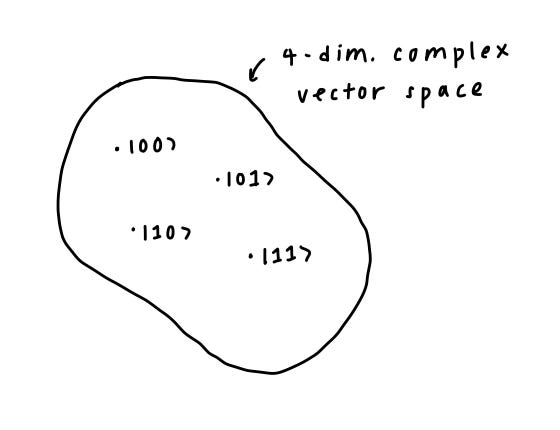
Why do we write the states in the way we do? When we consider the full space of two qubits, we have to take the tensor product of the two Hilbert spaces, which is one way of combining vector spaces mathematically. Thus, the four classical points, also the computational basis states of our system, are written as:
The state |00⟩ is shorthand for both qubit 1 and qubit 2 being in state |0⟩. The full Hilbert space of two qubits includes all valid superpositions of |00⟩, |01⟩, |10⟩, and |11⟩ in the same way that superposition applies to a single qubit.
Now we can add one more piece to the puzzle. When multiple qubits are present, entanglement is possible.
What’s entanglement? Quantum entanglement is a key principle at the heart of quantum cryptography and provides a potential quantum advantage in certain computing problems. Let’s dive in.
Entanglement
Conceptually, we can define entanglement as follows:
Entanglement is a phenomenon in quantum mechanics where two or more particles become interrelated or linked in such a way that acting on one immediately affects the state of the other, regardless of the distance between them.
The last part of the definition— regardless of the distance between them— is at odds with our intuition from classical physics of locality, or that things can only influence their immediate surroundings. This was so counterintuitive that Albert Einstein famously described entanglement as "spooky action at a distance" and (along with Podolsky and Rosen) came up with a model called hidden variable theory that explains entanglement in a way that obeys locality.
However, experimental results have provided concrete evidence that entanglement cannot be fully explained by hidden variable theory. In 1964, John Bell developed an inequality known as Bell’s theorem, which would be satisfied if hidden variable theory were true, and would be violated if the theory did not explain entanglement. Subsequent experiments violated these inequalities, showing concretely that this “spooky action at a distance” goes beyond what local hidden variable theory can explain. These experiments were honored with the 2022 Nobel Prize.
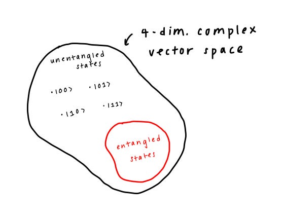
Fundamentally, entanglement means that we are not able to describe the entire system by the tensor product of its individual parts. In other words, the state of the entire system cannot be broken down into its individual qubits. Entangled states cover a portion of the state space and have special properties:
Let’s make this definition precise using some basic equations (don’t worry, we’ve distilled it down to basic algebra and systems of equations).
Mathematically Deriving Entanglement
Definition
Unentangled qubits means that the tensor product (combination) of the qubits are able to be decomposed into each individual qubit state.
Entangled qubits means that the tensor product (combination) of the qubits are NOT able to be decomposed into each individual qubit state.
In post 1, we defined all the states a qubit can be in by the following equation (where a and b are complex numbers where |a|2 + |b|2 = 1):
For a second qubit, we can just use different letters:
With multiple qubits, we take the tensor product of the two states of the qubits to generate the full state:
When each qubit is in the well-defined states above, we can write the following equation:
Now, let’s consider two scenarios with different values and see if solutions exist for a,b,c,d that satisfy the equation above.
Scenario 1
Let’s consider the scenario where ac = 1, ad = 1, bc = 1, and bd = 1 (forgetting normalization constraints).
In this case, there is a solution to this system of equations — a,b,c,d all equal 1. This means that the qubits are unentangled.
Scenario 2
Let’s consider another scenario where ac = 1, ad = 0, bc = 0, and bd = 1.
In this case, there exists no solution to this system of equations (there exists no a such as ac = 1, ad = 0, and bd = 1). This means that the qubits are entangled. This state is one example of the so-called Bell states, which are the maximally entangled states for 2 qubits. We’ll write them out here for reference:
Applications of Entanglement
The implications of entanglement are at the heart of the “second quantum revolution” that we alluded to in the last post. While important in all domains— sensing, simulation, computing, and networking — we’ll focus on quantum networking and communication today because the concepts can be understood at the level of two qubits.
In quantum communication, manipulating and distributing (usually entangled) quantum states over long distances and between separate quantum processors is the name of the game. Why do we care about transmitting and manipulating quantum information in this context? One application is cryptography — ways to make communication secure from unwanted parties. Today, we use something called public key, or asymmetric, encryption. At a high level, it works like this: say Sabrina wanted to send a secret message to Ryan. Ryan has a public key, or a string of information that will take a block of text and encode it into an indecipherable block of text. He also has a corresponding private key that only he knows, which will decode that message back into plain text. Sabrina would use Ryan’s known public key information to send the information over a public channel (where no one can view the original contents of the message), and Ryan would decode the message locally using his private key. These public and private keys are currently generated by RSA encryption, which leverages the NP-hardness of prime factorization.
Whether or not quantum computers will “break encryption”, quantum cryptography can theoretically establish verifiable, secure keys between parties. There are non-entanglement protocols and entanglement-based protocols. The entanglement-based one allows you to verify the presence of an eavesdropper by checking that Bell’s inequalities hold, which means that you could know from a physical measurement whether or not someone is trying to eavesdrop on you or not. This peer-to-peer protocol would allow any two parties to guarantee that their communication has not been tampered with. This could be applied to high-security military applications all the way down to civilian consumer communications. The generation of keys in this way is called Quantum Key Distribution (QKD).
Quantum Key Distribution (QKD)
There have been many exciting developments in QKD in the group of Jian-Wei Pan at the University of Science and Technology of China. Usually, quantum information is sent in the form of a photon through free space or an optical fiber between two processors, or nodes of a quantum network. Photons, often referred to as a good “flying qubit,” are a natural choice for a carrier of quantum information because they move quickly. One of the major technical limitations is the photon loss in free space and optical fibers; this places severe limitations on the physical distance that the nodes can be separated by while still establishing secure communication.
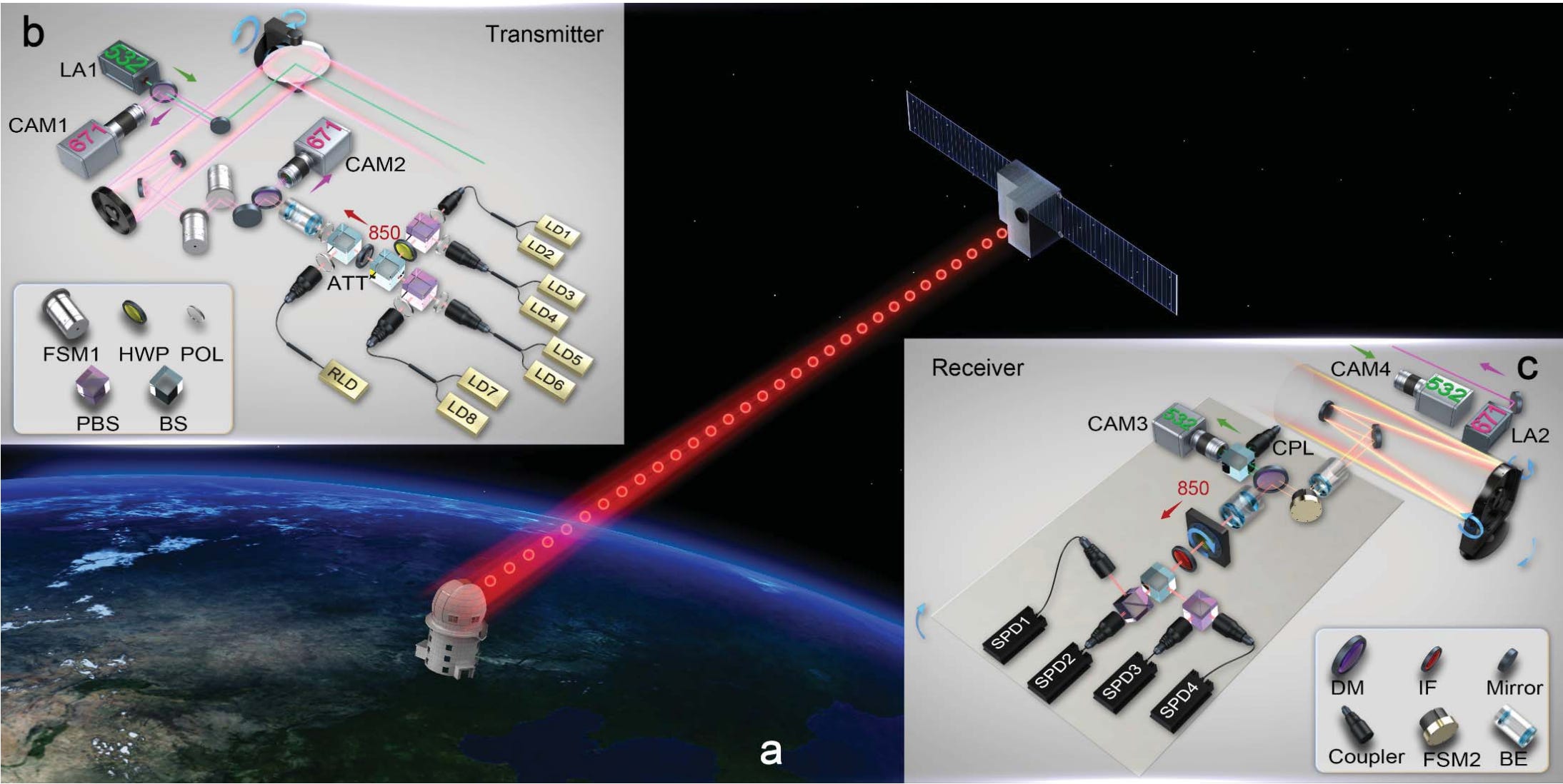
Pan and his group devised a solution that uses satellites in low-Earth orbit to extend the distance that two quantum nodes can talk to each other. Compared to the atmosphere on Earth, most of the atmosphere is free space and the effective thickness is much lower, leading to less photon loss. They launched a satellite named Micius into orbit, which passed by their node on the ground in Xinglong for approximately 5 min/day. In 2017, they implemented a non-entanglement-based QKD between a satellite and a ground station at Xinglong that was separated by over 1200 km, establishing a rate of ~1 kbit/sec key generation between the satellite and the ground node! This means that each second, they established 1000 bits that could potentially be used as a bit for a “secret key.” Below is a schematic of the satellite and the Xinglong ground station:
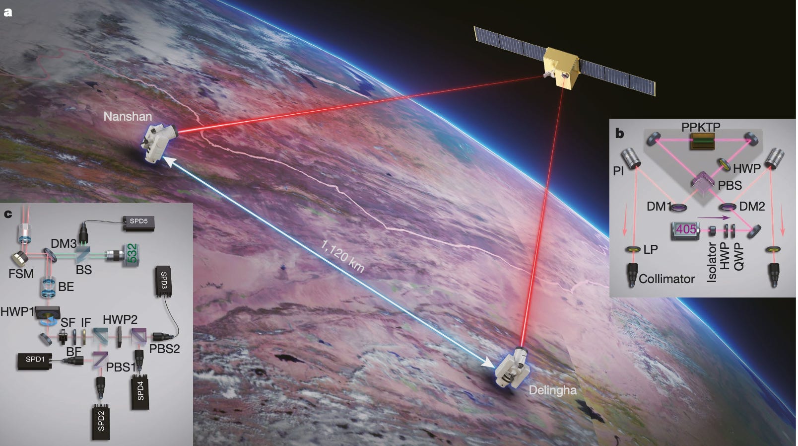
That same year, they also demonstrated that an entangled state generated on the satellite could be distributed between two ground nodes. This means that a laser on the satellite can generate entangled states of the photon’s polarization states (i.e. horizontal and vertical polarization states, if you remember this from your E&M physics classes). Then, they send one photon from the pair to each ground node, and tested the Bell inequalities that we talked about earlier to confirm that the photons were still entangled when reaching the ground. In 2020, they were able to build on this protocol by establishing entanglement-based QKD between two different ground nodes separated by 1120 km. By making drastic improvements to their experimental setup, which allowed them to improve their rate by a factor of 2 between the satellite and each of the ground nodes. Due to these upgrades, they achieved a post-selected key generation rate of 0.12 bits/sec.
A Lofty Goal
While these experiments are important developments in QKD, the vision of quantum networking also includes distributed computing, which requires a quantum computer (the ability to manipulate and store quantum information) at each node of the network. Fundamental operations include establishing entanglement between remote nodes (instead of the satellite generating one entangled pair locally and then sending each photon out to two different locations), quantum memory (storing quantum states), and quantum teleportation/state transfer (transferring information between nodes).
Remote Entanglement Generation
One experiment that has been working towards establishing entanglement between nodes is at the University of Innsbruck, Austria, in the groups of Tracy Northup and Ben Lanyon.
Their qubits of choice are ions, and in 2022, they were successful in entangling two ions separated by 230 m in different buildings. At each node, they define the qubit in two specific electronic states of an ion, then entangle each ion with a photon. Then, the photons travel through an optical fiber and interfere with each other, which can create correlations between the photons, which are already entangled/correlated with the ions. The photons are then measured, and they have engineered the system in a way such that certain measurement outcomes correspond to the ions being in the Bell states |𝚿+> and |𝚿-> that we’ve written above. Their success can be characterized by the entanglement generation rate, or how often they measure the certain outcomes that correspond to the Bell states, and the fidelity, or how close to a perfect Bell state the ions are actually in. Their entanglement generation rate is 0.43 sec-1, i.e. they generate on average 0.43 of those “good” measurements in one second, and their fidelity is on average 58.7%.
One of their biggest sources of error is that the photons need to be measured at the same time for ideal fidelity. If they restrict their measurements to a time window that is smaller, they achieve a rate of 3.1 min-1 and a fidelity of 88.2%. Overall, dealing with qubits that each have individual control systems in different buildings over such long distances is a complex undertaking, and this is an amazing scientific and engineering achievement. Other groups, including the QUANT-NET collaboration between the Department of Energy, Lawrence Berkeley National Lab, UC Berkeley, and Caltech are hoping to build on the foundations of this experiment.
Other Experiments
We sadly don’t have the time or space to go over every quantum networking experiment out there (there’s too much exciting work happening in the field!). However, other experiments focus on engineering systems that can act as quantum repeaters, which can help address the loss that occurs when sending photons through an optical fiber, thus increasing the distance at which quantum networks can exist. In addition, others are working on deterministic quantum state transfer and nonlocal operations between two nodes.
Wrapping Up
Even if all the math doesn’t make sense, we hope that you come away with a basic intuition of multiple qubit systems and entanglement. This provides the groundwork and context for at least some of the exciting stuff going on out there!
Thanks for reading. If anyone you know might be interested in this content, please share it. It helps a ton! Consider subscribing to have future posts delivered straight to your inbox: